Introduction

Whoooo boy. This one was a real challenge for me, an amateur computer engineer. As I was working through the issues in the IRQ Mistake, I realized that the real issue was much deeper than I had expected.

I spent the better part of two weeks attempting to figure out why my circuit (not that important as it turns out) was behaving as if one of the JK flip flops was transitioning in an “impossible” way.

It turns out, I didn’t know about something called “transmission line reflections”.

There Is No Perfect Square Wave

Electricty (both current and potential energy) behaves like a wave when a circuit changes the electricity in the circuit. This is a simple-enough statement, but it’s hard to appreciate the implications this has. Sure, a clock signal is definitely wave-like, but it is almost always modeled as a discrete stream of pulses. But everything is a wave, and the clock is no exception.

Without diving too deep into the innards of oscillators, partly because they are a bit beyond my depth of understanding, it’s sufficient to note that any thing that oscillates is producing some sort of wave.

It’s also important to note that things that produce waves, can never be truly digital. This is an annoying consequence of math, essentially. Or physics, depending on your philosophical views. Here’s a visualization of part of the problem:

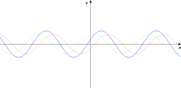
The red line is a square wave and the black line is the sum of 10 sine waves, each of which has an increasing frequency. The frequencies are chosen according to something called the Fourier Series, which is a way of approximating any function with a series of sine waves. And these frequencies that the Fourier series imposes are not random. They are the frequencies you get if you start at some base frequency and repeatedly increase the frequency through successive multiplication, i.e. \(f, 2f, 3f, ...\). You may have even heard of the names given to such frequencies: harmonics, a term that means the same thing in music :).

Note: There are more complexities to the actual Fourier Series than described above, but a deeper discussion would require significantly more math and I don’t think it’s necessary to understand the important operating principles.

When any oscillator oscillates, the resulting signal will always approximate a square wave pulse generator. Again, this is due to the fact that under the hood the oscillator is operating like a Fourier Series. With that in mind, let’s now consider how the oscillator can, and can’t, produce clock pulses.

Let’s imagine the electricity that a clock circuit produces. Let’s imagine that electricity starts at “0” and increases to its max value, which we’ll call “1”. As the oscillator approaches “1” it needs to stop increasing its electricity so it can flatten out at “1”:

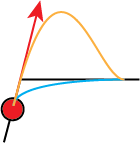
Reductively, the red point needs to either take something like the blue path or the orange path. This is because nothing can instantaneously alter its course/energy/eletricty/momentum. All things in nature require some time to change their path. You could even imagine the red dot has momentum according to the red arrow and note that momentum cannot change instantly.

The blue path won’t achieve the “1” value until after we might expect. The orange value does achieve the “1” value when we expect, but it then must compensate because it cannot instaneously stop at that value. If you play the orange trajectory in your mind, you’ll notice that it’s also possitble that there will be an oscillation as the orange line attempts to recover back and forth around the “1” value. You can see this exact phenomenon in the approximation we looked at:

This is not a coincidence. This is because oscillators (and most natural things) behave continuously like waves. Discontinuities, like the ones needed to produce a true square wave, tend to violate the rule above about changing direction/energy/etc instantaneously. And Fourier Series approximations work for continuous functions, all continuous period functions. These two phenomena (the continuity of the red dot’s path and the Fourier Series approximation to the square wave) are really the same exact phenomenon.

To see why it’s useful in this case to use the Fourier Series style of consideration, let’s crank up the number of terms in this approximation and see what happens when we try very hard to quickly hit “1” and stay there:

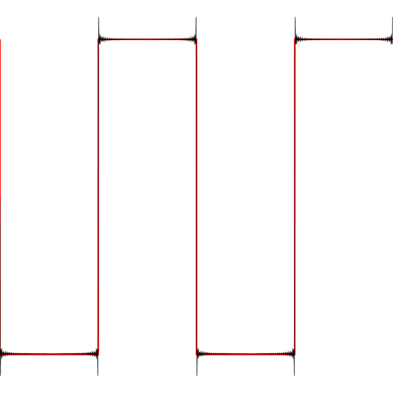
This is the exact same approximation (the Fourier Series one) with 300 terms instead of ten. We can never escape this! We must choose between three options:

1. The wave looks smoothed near the peaks, and arrives at those peaks later than expected.
2. The wave overshoots the peaks, and recovers slowly and smoothly to the peaks.
3. The wave overshoots the peaks, and oscillates around the peaks quickly settling on the peaks.

Option (2) is actually the same as (3) because there will always be some leftover energy to oscillate against, but for explanatory/intuitive purposes I find it’s helpful to separate them.

There are formal names for these, and wonderful physics reasons for them. Well, wonderful in the majestic sense. Not super for computer engineering as we’ll see. For a superb treament of these “damped oscillator” configurations, I highly recommend Hyper Physics’ explanation.

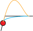
For completeness, this is what option (1) looks like, which is also called an overdamped oscillator:

Reflections

We’ve established that oscillators don’t actually produce clock pulses, but rather approximations to clock pulses via a Fourier Series approximation. Said differently, and now importantly, oscillators produce an infinite sum of waves, specifically a weighted sum of harmonics.

One thing most people have experience in their lives when it comes to waves is that they reflect off any discontinuity in the medium the wave is propagating through. Make some waves in the bath and when they hit the wall of the tub they will come back to you.

The oscillator is producing waves and thus those waves will reflect if they encounter a discontinuity in the medium they are propagating through. So the question is whether that happens in a circuit.

First we have to consider what the medium is that the oscillator waves are propagating through. It’s tempting to say it’s the copper traces, but that’s not quite true. The electricity itself is mediated by electrons flowing through the copper, and thus the waves are really waves of electric charge. If we break open some physics textbooks, or Google it, we’ll note that electric charge propagates through the electromagnetic field. Or we’ll find a very obtuse discussion about the philosophical meaning of fields and reality, but in this case we are going to stick to the electromagnetic field.

There are several things that can cause discontinuities in the electromagnetic field, but the important one (I think) here is a discontinuity in impedance. That kind of discontinuity is rampant at logic gate inputs because the impedance of those inputs is usually very high, especially compared to the impedence of the copper trace.

In effect, whenever the clock pulse from our oscillator encounters a logic gate input, the clock pulse will reflect back towards the clock source!

Standing Waves and Ringing

We have oscillators producing waves and gate inputs reflecting those waves back to the oscillator. This is a messy situation. It’s hard to describe exactly the result, but Wikimedia Commons has this rather nice animation for the approximate result:

Here we see a wave traveling to the right in red, the reflection traveling back to the left in green, and the resulting standing wave in blue.

Something similar happens in a circuit, but not exactly the same. The reflection is not perfectly elastic (i.e. some of the energy is lost), there is some impedance in the copper traces, and there are other factors I won’t pretend to understand. The net result is that for “long enough” traces, the wave is reflected back, a standing wave can be established (though not guaranteed), and a high frequency ringing artifact will appear on the line.

It seems to be somewhat of a rule-of-thumb situation that determines how long is “long enough”. I’m not able to find a definitive answer, but if I plug in the various parameters of the PCB for the Daughter Board into the KiCad Transmission Line Calculator, it tells me there is a “characteristic impedence” that is non-zero indicating this is an issue for us.

Perhaps more importantly, my oscilloscope doesn’t lie:

The bottom yellow line is the scope’s reading of the clock signal coming directly from the oscillator. The top cyan line shows clock signal on the clock line. There is clear pronounced ringing on the top line indicating that we’ve (inadvertently) created what’s called a transmission line, or any signal line that is long enough that ringing happens at the frequencies on that line.

All of this ringing is due to the oscillator producing waves, the implications of those waves (reflections), and the resulting emergent phenomenon. Phew.

Complex Problem, Easy Solution

There are a few ways to handle transmission line ringing, but the easiest seems to be to add a resistor at the source of the signal. The resistor will add impedance to the system, and if it’s chosen correctly can filter out the ringing produced in the line. This is where it’s helpful to switch back to the physics view of the world, because in effect we want to create a “Critically Damped Oscillator”. Such an oscillator will not exhibit ringing and will not take any longer to reach the maximum or minumum amplitude of the wave.

In the original diagrams, the critically damped oscillator is the one that produces the blue line:

Remember: everything is a wave! So this transmission line ringing is also a wave, and thus is also is an infinite sum of harmonics, and thus it will exhibit this overshoot/ringing unless it is critically damped.

Choosing the right value for the resistor is hard because it requires knowing about all of the impedences, inductances, capacitances, and the mathematical model relating them all to ringing. Fortunately, the KiCad Transmission Line Calculator seems to work reasonably enough, though it has its fair share of parameters that are hard to understand. In the end, the best way to choose a resistor value is to create an isolated experiment and adjust the resistor value until the signal reaches the critically damped trace.

In theory we would need to calculate this resistor value for every such clock trace and then have a resistor for each of them. That has two engineering issues:

1. It requires a separate trace for each clock signal
2. It requires a separate resistor for each trace

Instead, we can attempt to make all of the clock signal trace lengths about the same length and go with the Close Enough ™ argument.

Note: For traces like the D+/D- in USB signal lines it is much more important to get the trace lengths identical, but in this case close is good enough.

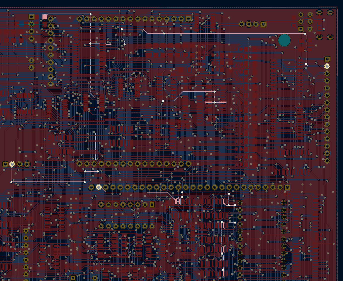
This is the trace for the CLK signal, originating in the top left. There are some branches, the results of which will create slightly different trace lengths to the various inputs, but again they’re Close Enough ™.

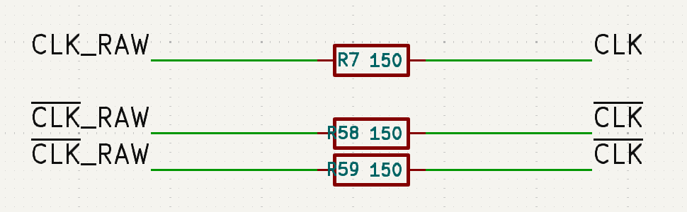
Plugging all of the values this trace length implies into the calculator it gives a transmission line resistance of about \(140\Omega\), but the closest resistor value that is common is \(150\Omega\), which again is Close Enough ™. The newest version of the Daughter Board has exactly those in it:

The Critically-Damped Oscillator

After all of this exposition and work the solution was simple: add a couple \(150\Omega\) resistors to a couple traces. Let’s see what the results of that simple, but profound, adjustment is.

This shows the difference, in the original circuit, between the clock signal coming directly from the clock (bottom, yellow) versus the signal on the CLK signal line (top cyan). There is clearly a lot of ringing. Consider the scale here is 2V per division (which is hard to see, apologies), and note that the ringing over/under shoots are nearly 2V in some places! That is more than enough to falsely trigger some TTL gate inputs.

This is the new CLK signal. It looks a little odd because this is actually a zoomed-in portion of the transition of the signal as it reaches that max (5V) level. Importantly, the scale for this image is 50mV instead of 2V, to show what little ringing there is. At the scale of the previous image this signal looked like a square wave. At this scale, there is a slight over-damping with very minimal ringing, which is expected because we know we’ll never perfectly get a square wave or even hit the magical critical damping in all cases.

One other minor point to note is that the rise and fall times of a critically-damped oscillator will necessarily be slightly slower than an under-damped one. This is due to the phenomenon described earlier about the energy needing to change “direction”. The cost for making a less-ringing signal is it slows down a bit. More precisely, it takes longer to reach its maximum value because the signal approaches it slowly to avoid the overshoot.

For completeness, the scope shows a rise time of \(26ns\) which comes out to about \(5.5ns/V\) if we use the displayed voltage range of \(4.73V\). This is well within the range of acceptable values for the logic families we’re using (see a laborious note about those acceptable values if you’re so inclined.).

Final Thoughts

It never occurred to me that I would need to understand the physics of electrical signal propagation so deeply when I started this project. I found myself in this position as I tried to explain behavior that didn’t make sense to me, namely in working on Integrating IRQ0 and the IRQ Mistake.

In those cases I started removing more and more assumptions about the circuit I was testing until I got to a place where there was only one conclusion left to draw: something was amiss with the clock signal. I set about attempting to deduce exactly what that something was. It was hard to figure this out as I am not a formally trained electrical engineer. I even posted to Stack Overflow.

Many of the folks on that thread pointed to noise in the power lines, which is definitely a problem, but was more of a red herring than anything. Through a lot of searching about how ringing could occur from a clock signal and searching about where undershoot and overshoot comes from I stumbled on the definition and considerations around “transmission lines”. The first formal note I discovered on this topic was in searching for information on how manufacturers advise engineers on proper implementation of oscillators.

Once I hypothesized the CLK signal was behaving like a transmission line, I fired up the oscilloscope in a very simple setup (to remove any confounding results) and confirmed this was the case. From there I started researching solutions and trying them out in my setup until I found a real solution.

This whole “adventure” was a good reminder about the importance of good engineering mixed with good science. That brackish point always seems to rear its head in a debugging setting. I find it fun; like trying to solve a very hard puzzle that definitely has a solution, but no one else has the answer to.

Remove assumptions. Simplify. Setup experiments. Use intuition. Read. Test. Validate. Repeat until there is only one answer left.